============================== \section*{A.2. Training ESM3}
\section*{A.2.1. Pre-training Data}
\section*{A.2.1.1. SEQUENCE DATAbASES}
UniRef release 202302 is downloaded and parsed from the official UniRef website (71). MGnify90 version 202302 is downloaded and parsed from MGnify (35). All nonrestricted studies available in JGI on July 31st, 2023 are downloaded and concatenated into the JGI dataset (72). OAS, which includes over a billion antibody sequences from
80 studies, is downloaded and clustered at $95 \%$ sequence identity (36).
\section*{A.2.1.2. CLUSTERING}
In all cases, data is clustered with mmseqs2 (73), with flags --kmer-per-seq 100 --cluster-mode 2 --cov-mode 1 -c 0.8 --min-seq-id $<$ seqid>.
In order to do cluster expansion, we separately cluster the dataset at the two levels, and perform a join to determine cluster member and cluster center based on IDs. We first sample a cluster center at the lower level, and then sample a sequence within the cluster at the higher level. As an example, for expansion of UniRef70 at $90 \%$, we first cluster UniRef at $70 \%$ sequence similarity using mmseqs linclust. Then, we cluster it separately at $90 \%$. Since each UniRef90 cluster center is by definition a UniRef70 cluster member, we filter out UniRef70 for all cluster members that are in the UniRef90 clusters. We can then drop all cluster centers without any members, which may occur due to the nondeterminism of clustering. This allows us to sample a UniRef70 center, and then a member within that cluster, of which each are $90 \%$ sequence similarity apart. For ease of dataloading, we additionally limit the number of data points within a cluster to 20 .
\section*{A.2.1.3. INVERSE FOLDING}
As data augmention we train a 200M parameter inverse folding model and use it to create additional training examples.
stack alternates between blocks with geometric attention and standard attention. The model is trained on the sequence and structure pairs in PDB, AlphaFold-DB, and ESMAtlas, with the single training task of (and loss computed on) predicting sequence at the output given structure at the input. Model architecture and training methodology is otherwise substantially similar to ESM3.
This model is used to generate additional sequences corresponding to each structure in the training data for ESM3 ( 5 sequences per structure for ESMAtlas and AlphaFold$\mathrm{DB}, 64$ sequences per structure for the $\mathrm{PDB})$. When training ESM3, with $50 \%$ probability the original sequence and structure pair is presented to the model as a training example. The other $50 \%$ of the time one of these 5 sequences is paired with the structure as the training example seen by ESM3.
\section*{A.2.1.4. FUNCTIONAL LABELS}
Functional labels are obtained from InterPro (38) and InterProScan (74), both version 95.0. All annotations for UniPro- tKB were downloaded from the InterPro website via the 'protein2ipr.dat.gz' file. InterProScan was applied to the entirety of MGnify 90 with flags --goterms --iprlookup --pathways --disable-precalc. The resultant values are taken as ground truth functional labels for model training.
\section*{A.2.1.5. STRUCTURAL DatA}
We use all PDB chains, clustered by unique PDB ID and entity ID within the PDB structure. We filter to all structures deposited before May 1, 2020, determined by X-ray crystallography, and better than $9 \AA$ resolution. (37)
s $<0.7$ pLDDT.
ESMAtlas is downloaded as version v0 and v2023_02. Similarly we use $\mathrm{a}<0.7$ pLDDT filter. We use a $0.7 \mathrm{pTM}$ cutoff as well to enforce globularity. High pTM structures tends to be more compact.
Structural data also includes any functional labels that exist for the corresponding sequence.
\section*{A.2.1.6. SolVent Accessible Surface AreA and SECONDARY STRUCTURE}
For solvent accessibility surface area, we use the ShrakeRupley rolling probe algorithm as implemented in biotite (75). This generates a set of real numbers, or a nan value when structural coordinates are not provided. Similarly, SS8 labels are generated using the mkdssp tool (76) and taken as ground truth labels.
In both cases, we use the set of high quality predicted structures in AlphaFoldDB and ESMAtlas. We split our datasets into structural and sequence data. Structural data is shown separately in order to weight the ratios of structural data (mostly synthetic) properly with the amount of sequence data (mostly real).
An oversight was that we did not manage to apply these augmentations to PDB. However, since PDB constituted a relatively small portion of our training data, and these structural conditioning tasks did not depend on precise sidechain positions, we reasoned that high confidence synthetic structures would perform equally well and annotation of PDB was not necessary.
\section*{A.2.1.7. PURGING of VALIDATION SEQUENCES}
.8 {cov-mode 0 --max-seqs 300 --max-accept 3 --start-sens 2 -s 7 --sens-steps 3.
This query is designed such that early stopping in mmseqs will not affect if we find a hit in the "query" training set.
Train purges are run to generate a list of blacklisted UniRef, MGnify, and JGI IDs, which are removed from the training set.
\section*{A.2.1.8. TOKEN COUNTS}
The dataset counts in Table S3 are computed after limiting the large clusters to 20 . The number of tokens are computed by multiplying the number of sequences with the average length of the dataset.
In order to compute the approximate number of sequences and tokens seen during training, we first compute the number of times the dataset is repeated at the cluster level. Given the the number of repeats, we know the expected number of unique samples seen when sampling with replacement is $n\left(1-\left(1-\frac{1}{n}\right)^{k}\right)$ with a cluster of size $n$ and $k$ items selected. Computing this on the size of each cluster and number of dataset repeats results in the approximate number of tokens we present as presented in Table S4. Our largest model is trained on all of this data, while our smaller models use a portion of it depending on the model's token budget.
\section*{A.2.2. Pre-training Tasks}
\section*{A.2.2.1. NOISE SCHEDULE}
In the masked generative framework, corruption is applied to each input to the model. To enable generation, the amount of noise applied to an input is sampled from a distribution with probability mass on all values between 0 and 1 .
We select various noise schedules for different tracks with several goals in mind. First, ESM3 should see all combinations of tracks as input and output, enabling it to generate and predict based on arbitrary inputs. Second, ESM3 should maintain a balance of strong representation learning and high quality generations. Third, the type of inputs provided should be representative of what users would like to prompt the model with.
entation, we found that a fixed $15 \%$ noise schedule led to poor generation results, while a linear noise schedule where probability of each mask rate was constant led to good generation but poor representation learning results. We find a good trade-off between representation learning and generation by sampling the noise schedule from a mixture distribution. $80 \%$ of the time, the mask rate is sampled from a $\beta(3,9)$ distribution with mean mask rate $25 \%$. $20 \%$ of the time, the mask rate is sampled from a uniform distribution, resulting in an average overall mask rate of $30 \%$.
The noise schedules applied to each input are listed in Table S6. For the structure coordinate track, we also modify the noise to be applied as span dropping, as opposed to i.i.d over the sequence with $50 \%$ probability. This ensures that the model sees contiguous regions of masked and provided coordinates, which better mimics the types of inputs users may provide.
\section*{A.2.2.2. TRaCK DRoPOUT}
Along with applying noise to each track, we want to ensure ESM3 is able to perform well when some tracks are not provided at all (e.g. to perform structure prediction when no structure is provided as input). We enable this by wholly dropping out some tracks with varying probabilities, listed in Table S6.
\section*{A.2.2.3. StRUCTURE NOISE}
We apply gaussian noise with standard deviation 0.1 to all coordinates the model takes as input.
\section*{A.2.2.4. ATOMIC CoORdinATION SAMPLING}
tter perform the type of atomic coordination required for active site sampling.
While this task will be sampled with some probability under the standard noise schedules, we also manually sample the task with $5 \%$ probability whenever a structure is available. If the task is sampled and a valid atomic coordination triplet is found, the structure coordinates for that triplet are shown to the model. For each residue in the triplet, the adjacent residues are also independently shown with $50 \%$ probability, which leads to a total size of between 3 and 9 residues. All other structure coordinates are masked. Normal masking is
\begin{tabular}{ccccll} \hline Dataset & Type & Clustering Level & Expansion Level & Tokens & Release \ \hline UniRef & Sequence & $70 \%(83 \mathrm{M})$ & $90 \%(156 \mathrm{M})$ & $54.6 \mathrm{~B}$ & $2023 _02$ \ MGnify & Sequence & $70 \%(372 \mathrm{M})$ & $90 \%(621 \mathrm{M})$ & $105.5 \mathrm{~B}$ & 202302 \ JGI & Sequence & $70 \%(2029 \mathrm{M})$ & - & $256 \mathrm{~B}$ & All non-restricted studies available on \ & & & & & July 30th, 2023. \ OAS & Sequence & $95 \%(1192 \mathrm{M})$ & - & $132 \mathrm{~B}$ & All sequences available on July 30th, \ & & & & & 2023. \ PDB & Structure & $-(203 \mathrm{~K})$ & - & $0.054 \mathrm{~B}$ & All chains available on RCSB prior to \ PDB Clustered & Structure & $70 \%(46 \mathrm{~K})$ & $100 \%(100 \mathrm{~K})$ & $0.027 \mathrm{~B}$ & May, 1st, 2020 \ AlphaFoldDB & Structure & $70 \%(36 \mathrm{M})$ & $90 \%(69 \mathrm{M})$ & $40.5 \mathrm{~B}$ & v4 \ ESMAtlas & Structure & $70 \%(87 \mathrm{M})$ & $90 \%(179 \mathrm{M})$ & $23.5 \mathrm{~B}$ & v0, v202302 \ \hline \end{tabular}
Table S3. Pre-training dataset statistics. Includes number of tokens, release, and clustering level. Numbers are derived after dataset filtering.
\begin{tabular}{ccc} \hline Dataset Name & Unique Samples(M) & Unique Tokens(M) \ \hline UniRef & 133 & 40,177 \ MGnify & 406 & 65,780 \
\ OAS & 203 & 22,363 \ PDB & 0.2 & 55 \ AFDB & 68 & 20,510 \ ESMAtlas & 168 & 38,674 \ AFDB inverse folded & 111 & 33,300 \ ESMAtlas inverse folded & 251 & 57,730 \ \hline Sequence & 3,143 & 484,441 \ Structure & 236 & 177,710 \ Annotation & 539 & 105,957 \ \hline Total unique training tokens & & 768,109 \ \hline \end{tabular}
Table S4. Pre-training unique token statistics. Broken down by token type and dataset type.
\begin{tabular}{rcccc} \hline Dataset & Inverse Folding & Function Labels & SASA & Secondary Structure \ \hline UniRef & $\checkmark$ & $\checkmark$ & - & - \ MGnify & $\checkmark$ & $\checkmark$ & - & - \ JGI & $x$ & $x$ & - & - \ OAS & $x$ & $x$ & - & - \ PDB & $x$ & $x$ & $x$ & $\mathbb{\checkmark}$ \ AlphaFoldDB & $\checkmark$ & $\checkmark$ & $\checkmark$ & $\checkmark$ \ ESMAtlas & $\checkmark$ & $\checkmark$ & $\checkmark$ & $\checkmark$ \ \hline \end{tabular}
Table S5. Data augmentation and conditioning information applied to each dataset.
\begin{tabular}{lll} \hline Track & Noise Schedule & Dropout Prob \ \hline Sequence & betalinear30 & 0 \ Structure Tokens & cosine & 0.25 \ Structure Coordinates & cubic & 0.5 \ Secondary Structure (8-class) & square root & 0.9 \ SASA & square root & 0.9 \ Function Tokens & square root & 0.9 \ Residue Annotations & square root & 0.9 \ \hline \end{tabular}
Table S6. Noise Schedules and Dropout Probabilities.
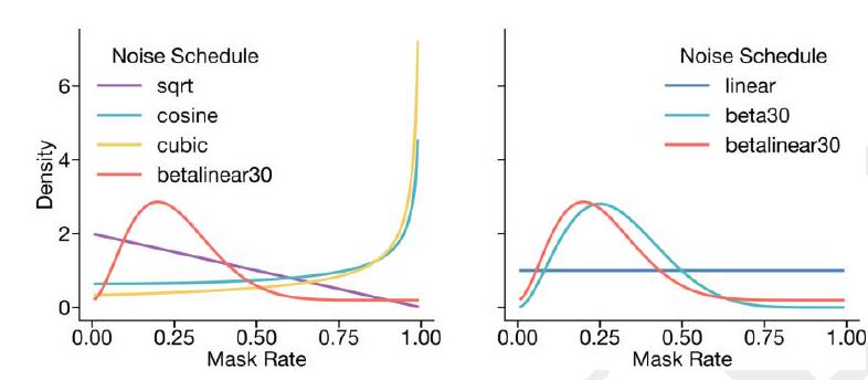
Figure S9. Visualization of noise schedules used. Left shows the probability density function of all noise schedules used. Right shows the betalinear30 distribution (which is drawn from $\beta(3,9)$ with $80 \%$ probability and a linear distribution with $20 \%$ probability) against a beta30 distribution (defined by $\beta(3,7)$ ) and a linear distribution.
applied to the other tracks.
\section*{A.2.2.5. TERTIARY INTERFACE SAMPLING}
nd generating binding interfaces is another important task for generative protein models. To help with this capability, we add computational data augmentation that simulates the binding interface task.
We define a tertiary interface as one involving a long range contact $(C \alpha-C \alpha$ distance $<8 \AA, \geq 24$ sequence positions). When this task is sampled ( $5 \%$ probability whenever a structure is present), a long range contact is found, then the chain is split into two chains, each containing one side of the contact interface. Suppose the contacting positions are given by the indices $i, j$. Then the first chain will contain residues between [RANDINT $(1, i-3)$, RANDINT $(i+3, j-15)$ ], while the second chain will contain residues between [RANDINT $(i+15, j-3)$, RANDINT $(j+15, L)$ ]. This ensures there is always a residue gap between the two pseudochains. A chainbreak token "-" is inserted to represent the residue gap.
\section*{A.2.2.6. ReSIDUE GAP AUGMENTATION}
To encourage the model to learn to represent residue gaps using the chainbreak token, we introduce a task which randomly splits a single chain into multiple subchains.
First, a number of chains to sample is sampled from a geometric distribution with probability 0.9 , up to a maximum of 9 possible chains. If the number of chains sampled is 1 , no additional transformations are applied. A minimum separation of 10 residues between chains is defined. Sequence lengths of the chains along with gaps are sampled from a dirichlet distribution to maintain identically distributed sequence lengths for each chain. This transformation is applied to all samples.
\section*{A.2.2.7. GEOMETRIC ATTENTION MASKING}
known, but the interface is unknown.
\section*{A.2.3. Training Details}
\section*{A.2.3.1. HYPERPARAMETERS}
We train all models using AdamW optimizer (77), with the following hyperparameters: $\beta{1}=0.9, \beta{2}=0.95$. We use a weight decay of 0.01 and gradient clipping of 1.0. We employ $5 \mathrm{~K}$ to $20 \mathrm{~K}$ warmup steps until reaching the maximum learning rate, and utilize a cosine decay scheduler to decay LR to $10 \%$ of the maximum learning rate by the end of training.
\section*{A.2.3.2. INFRASTRUCTURE}
Our training codebase uses Pytorch. We use Pytorch's FSDP (78) implementation for data parallelism. We also use custom components from the TransformerEngine (79) library.
We have made several optimizations to increase the training speed of our models. For multi-head attention uses, we use the memory efficient implementation from the xformers library (80). We also save activations that are expensive to compute during training when necessary. We employ mixed precision training, utilizing FP8, BF16, and FP32 as needed based on accuracy requirements and kernel availability throughout our network.
\section*{A.2.3.3. StABILITY}
Scaling ESM3 to 98 billion parameters with its novel architecture, multi-modal inputs, and low precision computation requirements poses significant training stability challenges. Our model is significantly deeper than its NLP counterparts, and literature has shown that deeper networks are harder to train due to attention collapse (81).
le biased towards lower mask rates improved both performance and training stability. Interestingly, the introduction of conditioning from other modalities also improves training stability, perhaps suggesting that stability is related to the degree of underspecification of a task.
An incorrectly set learning rate is another source of instability. To ensure the right balance between learning effectiveness and stability, we optimized the learning rate on smaller models and scaled it according to best practices as outlined in $(84,85)$. We find empirically that the initialization has a small effect on model stability, and the majority of stabilization can be gained from simply scaling the learning rate at the appropriate rate. By applying the rules in both width $-\mu \mathrm{P}$ and depth $-\mu \mathrm{P}$, we can simply scale the learning rate inversely proportional to the square root of the number of parameters, and find this results in stable training.
Following these modifications, we successfully trained our 98-billion-parameter model without any issues related to training instability.
\section*{A.2.3.4. STAGED TRAINING}
We stage training to alter dataset composition, train on longer contexts that would be too expensive for the entire pre-training, or introduce features such as the taxonomy track (A.1.9.2.