============================== \section*{A.3. Model evaluations}
ESM3 is both a generative model and a representation learning model that can be adapted for predictive tasks. In this section, we present benchmarking results for both capabilities.
\section*{A.3.1. Models}
ESM3 models are trained at three scales-1.4B, 7B, and 98B parameters-on approximately 75B, 560B, and 1.8T training tokens, respectively.
The ESM3 1.4B model, trained on 75B tokens and noted for its small size and speed, allows rapid iteration both during training and at inference. Optimal model size and number of training tokens are studied by extrapolating from a series of smaller runs, given a training compute budget, model architecture, and dataset characteristics $(19,21)$. After determining compute optimality for training, a variety of factors such as release frequency, amount of inference, ease of use, and usage patterns are also taken into account to determine the ideal number of tokens on which to train the model. To enable efficient inference for the benefit of the research community, we have trained two additional versions of ESM3 1.4B, named 1.4B Overtrained and 1.4B Open, which are trained on 300B tokens, far beyond their compute optimality for training.
\section*{A.3.2. Data}
In the following benchmarks for this section, unless otherwise noted, models are evaluated on a test set of 902 proteins whose structures are temporarily held out from the ESM3 training set. The proteins were sourced from the Continuous Automated Model EvaluatiOn (CAMEO) targets released from May 1, 2020 through Aug 1, 2023 (86).
For contact and structure prediction evaluations, we also evaluate on the CASP14 (71 proteins) and CASP15 (70 proteins) structure prediction benchmarks $(87,88)$. The CASP14 and CASP15 sets are obtained directly from the organizers.
\section*{A.3.3. Representation Learning}
pair, outputting the probability of contact between them. We use LoRA (89) for finetuning, which is a common alternative to full weight finetuning that uses much less memory while attaining strong performance. LoRA is applied to the base model for finetuning, and the MLP along with the LoRA weights are trained end-to-end using the cross-entropy loss with respect to the ground truth contact prediction map. For the ground truth, all residues at least 6 positions apart in the sequence and within an $8 \AA$ $\mathrm{C} \alpha$ - $\mathrm{C} \alpha$ distance are labeled as a contact. All models are trained with LoRA rank 4, batch size 64 and a learning rate of $1 \mathrm{e}-3$ for $10 \mathrm{k}$ steps on a mix of sequence and structure data from PDB, AlphaFold-DB, ESMAtlas, and OAS Predicted Structures. Data are sampled in a ratio of 1:3:3:0.03 from these datasets.
Table S7 shows the performance on each structural test set through the metric of precision at $\mathrm{L}(\mathrm{P} @ \mathrm{~L})$, which evaluates the precision of the top- $\mathrm{L}$ most confident predictions, where $\mathrm{L}$ is the length of the protein. The smallest ESM3 model, with 1.4B parameters, achieves a $\mathrm{P} @ \mathrm{~L}$ of $0.76 \pm 0.02$ on the CAMEO test set, which is higher than the $3 \mathrm{~B}$ parameter ESM2 model $(0.75 \pm 0.02)$. Furthermore, it trains on an order of magnitude less compute during pre-training ( $6.72 \times$ $10^{20}$ FLOPS vs. $1.8 \times 10^{22}$ FLOPS), demonstrating the benefits of multimodal pre-training.
\section*{A.3.4. Structure Prediction}
ESM3 can directly predict protein structures without additional finetuning by first predicting structure tokens, then decoding these tokens into coordinates. When predicting structure tokens, we follow the strategy outlined in Appendix A.1.10 and test both argmax decoding and full iterative decoding.
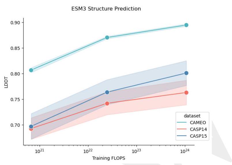
le S8), whereas for easier datasets like CAMEO, argmax prediction is sufficient. On both the CAMEO and CASP15 datasets, argmax prediction for the 7B model is comparable to ESMFold, and iterative decoding with ESM3 98B closes the gap between ESMFold and Alphafold2. Structure prediction scaling curves as a function of training compute, are provided in Fig. S10
\section*{A.3.5. Conditional Likelihood}
The conditional likelihood of an output given a prompt serves as a proxy for the generative capabilities of a model. Fig. S11 and Table S9 evaluate the performance of ESM3 as a conditional generative model, using its negative log likelihood (NLL) on the test set. For each track - sequence, structure, function, SASA, and secondary structure - NLL is evaluated both unconditionally and conditioned on each of the other tracks.
Figure S10. Scaling curves for structure prediction. Error bars are single standard deviations.
Unlike, for example, an autoregressive model, ESM3 is a generative model over masking patterns, so is trained to predict tokens given any masking pattern. The NLL of a sample under ESM3 is given by $\frac{1}{L!} \sum{o \in \mathbb{O}} \frac{1}{L} \sum{i=1}^{L} \log p\left(x{o{i}} \mid x{o{1}}, \ldots, x{o{i-1}}\right)$, where $O$ is the set of all decoding orders with normalization constant $Z=\frac{1}{L!}$. This computation is intractable (as the set of all decoding orders is exponential in length of a protein), but can be approximated by sampling a single decoding order $o$ for each $x$ in our dataset. At each step teacher forcing is used to replace the masked token with the ground truth token and report the mean NLL over the output tokens.
3 \mathrm{D}$ structure reduces the loss on secondary structure prediction to nearly zero (1.4B: $0.24,7 \mathrm{~B}: 0.19,98 \mathrm{~B}: 0.16$ ).
Other trends may be more surprising. Conditioning on sequence results in a lower structure prediction loss than conditioning on secondary structure (98B; sequence: 3.13 , secondary structure: 3.37). There are some diminishing returns to scale for the prediction of structure, function, SASA, and secondary structure. However, this diminishing is not observed for sequences, where we observe a clear loglinear relationship between pre-training FLOPS and NLL, regardless of conditioning.
\section*{A.3.6. Unconditional Generation}
To assess the model's unconditional generation capability, we sampled 100 protein lengths randomly from the PDB and generated 1,024 sequences for each using ESM3 98B with a constant temperature of 0.7 . The sampled length distribution is shown in Fig. S13A. Structures for each sequence were predicted using ESM3 7B, and the distribution of pTM
\begin{tabular}{|c|c|c|c|} \hline Model & CASP14 & CASP15 & CAMEO \ \hline ESM2 3B & $0.57(0.49-0.64)$ & $0.57(0.48-0.65)$ & $0.75(0.73-0.77)$ \ \hline ESM3 1.4B & $0.56(0.48-0.64)$ & $0.59(0.50-0.66)$ & $0.76(0.74-0.78)$ \ \hline ESM3 7B & $0.62(0.54-0.70)$ & $0.64(0.56-0.73)$ & $0.82(0.80-0.84)$ \ \hline ESM3 98B & $0.66(0.57-0.74)$ & $0.66(0.57-0.75)$ & $0.85(0.83-0.86)$ \ \hline \end{tabular}
Table S7.Precision @ L results. Measured on CASP14, CASP15 and CAMEO for the ESM3 model family. Intervals represent bootstrapped $95 \%$ confidence intervals.
\begin{tabular}{c|ccc|ccc} & \multicolumn{3}{|c|}{ Iterative $/ O\left(L^{3}\right)$} & \multicolumn{3}{c}{$\operatorname{Argmax} / O\left(L^{2}\right)$} \ Model & CAMEO & CASP14 & CASP15 & CAMEO & CASP14 & CASP15 \ \hline 1.4B Open & 0.830 & 0.705 & 0.733 & 0.805 & 0.640 & 0.677 \ 1.4B Overtrained & 0.846 & 0.714 & 0.750 & 0.825 & 0.651 & 0.700 \
0.636 \ 7B & 0.870 & 0.742 & 0.764 & 0.852 & 0.607 & 0.726 \ 98B & 0.895 & 0.763 & 0.801 & 0.884 & 0.719 & 0.770 \ \hline ESMFold & 0.865 & 0.728 & 0.735 & & & \ AlphaFold2 & 0.904 & 0.846 & 0.826 & & & \end{tabular}
Table S8. Protein structure prediction results. We benchmark ESMFold, ESM3 models, and Alphafold2. Left side: ESM3 iterative inference of structure tokens conditioned on sequence. Because iterative inference is $O\left(L^{3}\right)$ in length of a protein sequence, it is comparable to ESMFold and AF2, both of which share the same runtime complexity. Right panel: Single-pass argmax structure token given sequence. In all cases, the more difficult the dataset, the more iterative decoding appears to help - 98B has a +4.4 LDDT boost on CASP14, compared to a +1.0 LDDT boost on CAMEO. Both the Open and Overtrained models are both trained up to 200k steps. The plain 1.4B model is used for scaling comparisons, and is trained to $50 \mathrm{k}$ steps.
\begin{tabular}{cc|ccccc} & & \multicolumn{5}{|c}{ Conditioning } \ & Model & Sequence & Structure & Function & SASA & Secondary Structure \ \hline & $1.4 \mathrm{~B}$ & 2.31 & 1.71 & 2.28 & 1.81 & 2.02 \ Sequence & $7 \mathrm{~B}$ & 2.04 & 1.43 & 2.00 & 1.47 & 1.74 \ & 98 & 1.84 & 1.21 & 1.76 & 1.21 & 1.50 \ & $1.4 \mathrm{~B}$ & 4.09 & 4.98 & 4.93 & 4.39 & 4.42 \ Structure & $7 \mathrm{~B}$ & 3.42 & 4.2 & 4.18 & 3.62 & 3.71 \ & 98 & 3.13 & 3.85 & 3.8 & 3.24 & 3.37 \ & $1.4 \mathrm{~B}$ & 1.81 & 1.98 & 4.52 & 2.29 & 2.24 \ Function & $7 \mathrm{~B}$ & 1.22 & 1.47 & 3.75 & 1.67 & 1.70 \ & 98 & 0.93 & 1.20 & 3.63 & 1.41 & 1.40 \ & $1.4 \mathrm{~B}$ & 1.78 & 1.81 & 2.42 & 2.48 & 2.10 \ SASA & 7B & 1.57 & 1.66 & 2.26 & 2.31 & 1.92 \ & 98 & 1.46 & 1.56 & 2.15 & 2.23 & 1.82 \ Secondary & $1.4 \mathrm{~B}$ & 0.42 & 0.24 & 0.70 & 0.50 & 0.83 \ Structure & $7 \mathrm{~B}$ & 0.31 & 0.19 & 0.57 & 0.31 & 0.6 \ & 98 & 0.26 & 0.16 & 0.50 & 0.25 & 0.54 \end{tabular}
ch track conditioned on other tracks. Each row is a model size, generating a particular modality. Each column is the conditioning. The diagonal, highlighted with italics, are the unconditional NLL of each track. We observe that indeed adding conditioning improves NLL in all cases.
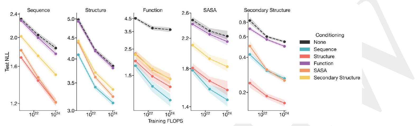
Figure S11. Conditional and unconditional scaling behavior for each track. Loss is shown on CAMEO (Appendix A.3.2
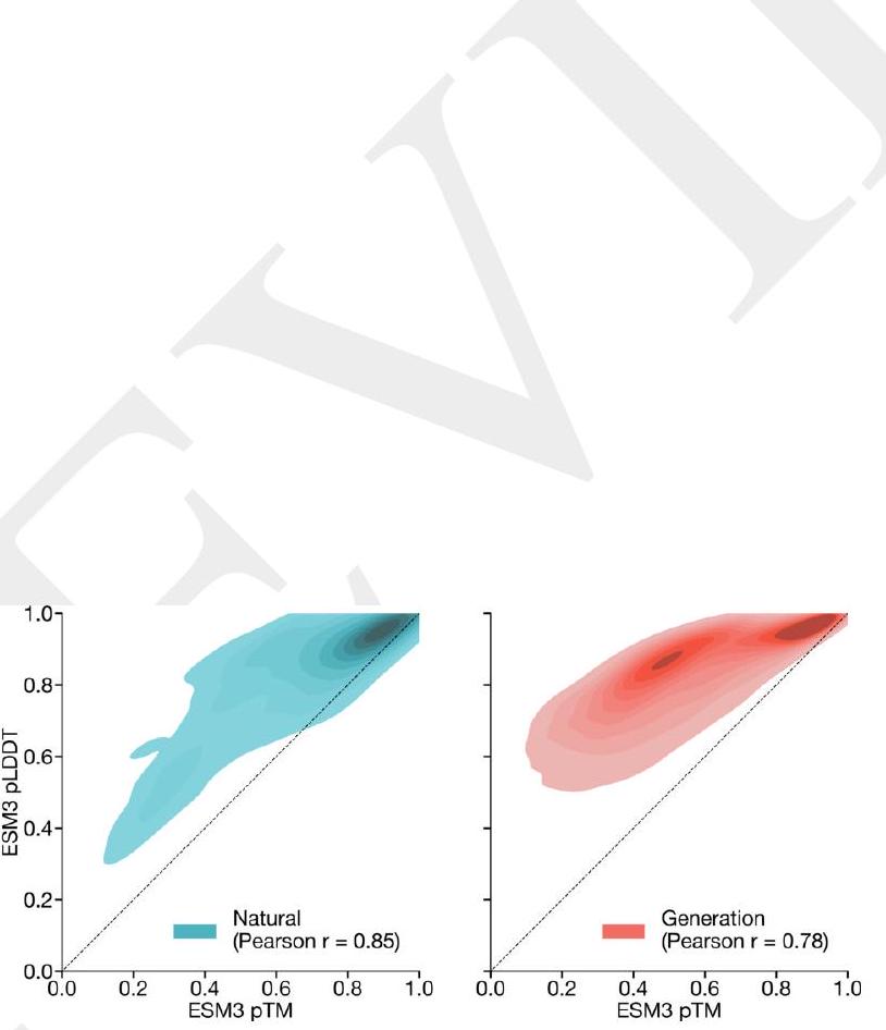
Figure S12. Distribution of $p T M$ and $p L D D T$. Measured on natural (left) and generated (right) sequences under ESM3 7B structure prediction. Generated sequences show a clearly lower correlation (Pearson $\mathrm{r} 0.79 \mathrm{vs}$. 0.85 ) as well as a mode of sequences with high pLDDT but low pTM. Natural sequences are from the test set (Appendix A.3.2), generations are unconditional generations from ESM3 98B. and pLDDT are shown in Fig. S13B. ESM3 generates more high-quality structures than ESM2, which was trained using a simple MLM objective over sequence only with a fixed mask rate. Sequence similarity to the training set was computed using mmseqs2 (73) with the following parameters: --cov-mode 2 -c 0.8 -s 6.0. Proteins generated unconditionally are similar-but not identical-to proteins found in the training set (Fig. S15) and have high coverage of the training set (Fig. 1E), demonstrating that the model has properly fit the training distribution and does not exhibit mode collapse. We observe a cluster of generations with very high sequence identity to the training set; these correspond to antibody sequences, with the framework regions accounting for the high sequence identity.
structures and can overestimate the confidence of a prediction. pLDDT is biased towards local structural confidence, which can result in pathologies such as very long alpha helices with high pLDDT at all positions. pTM is a more global measure of structural confidence, and is more robust to these pathologies. Fig. S12 shows that $\mathrm{pTM}$ and pLDDT correlation drops for generated sequences $($ Pearson $\mathrm{r}$ : natural $=0.85$, generation $=0.79$ ), and a clear pattern of high pLDDT ( $>0.8$ ) but low pTM $(<0.6)$ emerges.
To visualize the distribution of unconditional generations, we compute sequence embeddings by extracting the final layer outputs produced by running ESM3 7B with sequence inputs only. Protein-level embeddings are computed by averaging over all positions in the sequence to produce a 2560 -dim embedding. We then project these embeddings into two dimensions using a UMAP projection (90) fit on a background distribution of 50,000 randomly sampled sequences from UniProt with minimum distance 0.1 and number of neighbors 25 . Examples are selected by computing structural clusters with Foldseek-cluster (using default parameters) and sampling the example with highest ESM3 pTM from each cluster. A subset of these cluster representatives are shown in Fig. 1E.
ma- jority of generations successfully re-folded with TM-score of greater than 0.8 to the hallucinated structures, demonstrating that ESM3 has high self-consistency for its own high-confidence designs (Fig. S13C).
To explore alternative ways of generating proteins, we assess the quality of proteins generated by a chain-of-thought $(\mathrm{CoT})$ procedure in which ESM3 7B generates the secondary structure (SS8 tokens), then the 3-D backbone coordinates (structure tokens), followed by the amino acid sequence (sequence tokens) (Fig. S14). We compare the quality of amino acid sequences generated from this CoT procedure with the above method of unconditionally directly generating amino acid sequences. We find that the CoT procedure generates sequences that have higher confidence ESM3predicted structures than the directly-generated sequences as measured by pTM and mean pLDDT (Fig. S14A). Compared to high-confidence ( $\mathrm{pTM}>0.8$, mean $\mathrm{pLDDT}>0.8$ ) directly-generated sequences, the high-confidence subset of CoT-generated sequences are also more designable: the CoT-generated sequences have predicted structures whose inverse folded, then re-refolded structures have higher TMscore to the originally predicted structure (Fig. S14C). The CoT-generated sequences show a small bias towards higher alpha and beta proportion compared to those generated directly (Fig. S14D).
\section*{A.3.7. Prompt-following Evaluations}
xample, for the structure track, for a protein of length 100 , we may sample a random span of 15 residues from residue $20-35$. The model would then have to generate a protein sequence of length 100 conditioned on structure coordinate conditioning from residues 20-35 derived from the original test protein. This same procedure is applied for the secondary structure and SASA tracks. For the function track, we form the prompt by tokenizing the keywords form the InterProScan annotations associated with each sequence. The ESM3 7B model is used for all generations with a temperature of 0.7 and $L$ decoding steps (where $L$ is the length of the sequence). The model generates 64 sequences per prompt, which we use to compute pass64.
To evaluate the generations, we use ESMFold to fold the sequences generated by ESM3. For the structure coordinate, secondary structure, and SASA tracks, the relevant align-
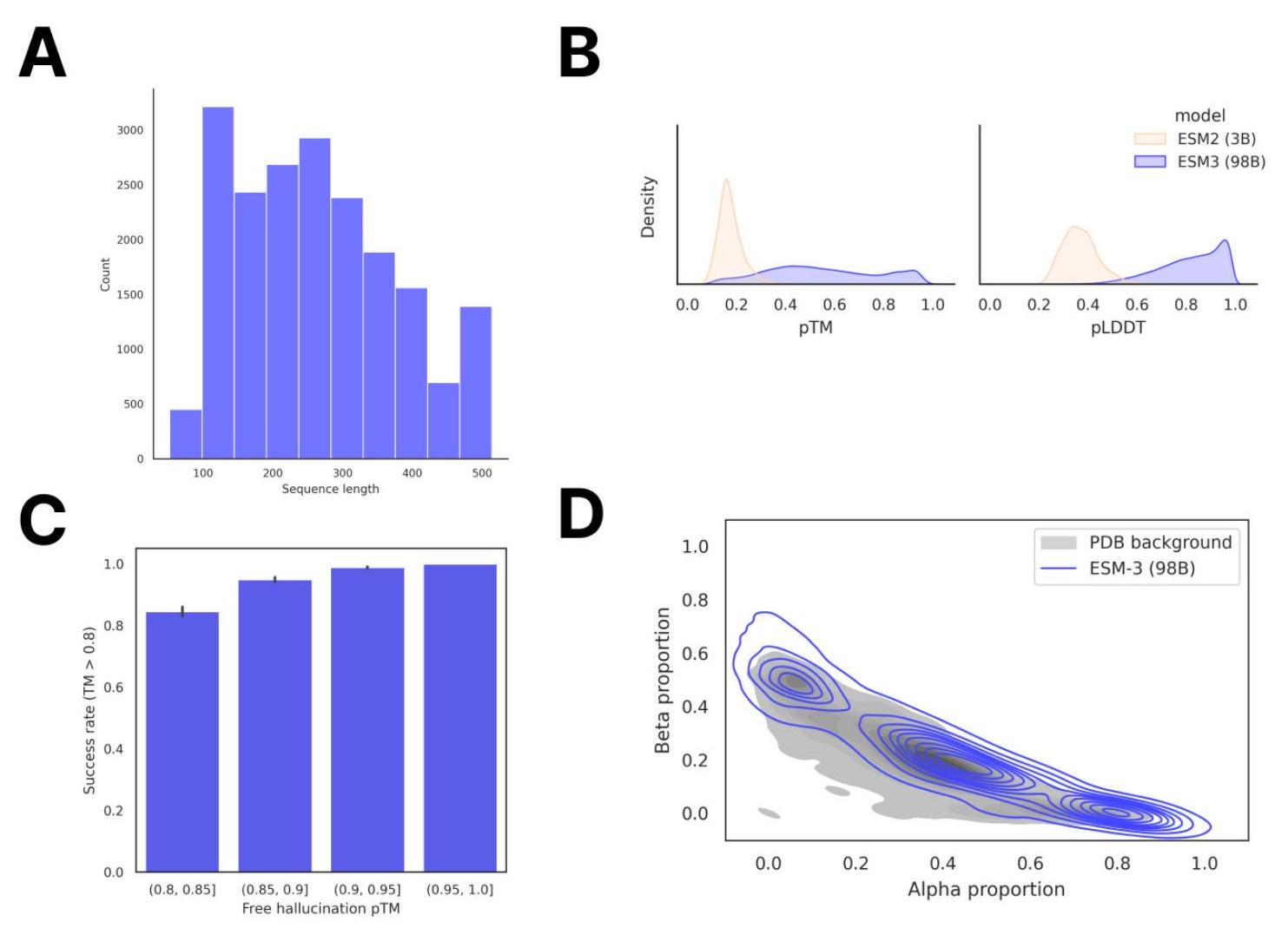
Figure S13. Unconditional generation of high-quality and diverse proteins using ESM3. (A) Distribution of sequence length in the unconditional generation dataset. (B) Mean pLDDT and pTM of unconditional generations from ESM3 compared to sequences designed using the 3B-parameter ESM2 model. (C) Round-trip success rate of high-confidence generations using ESM3. Predicted structures were inverse folded to predict a new sequence and then re-folded to produce a new structure. Success was measured by a TM-score of greater than 0.8 between the original and refolded designs. (D) Secondary structure composition of unconditional generations relative to the distribution of proteins in the PDB, which is shown in gray.
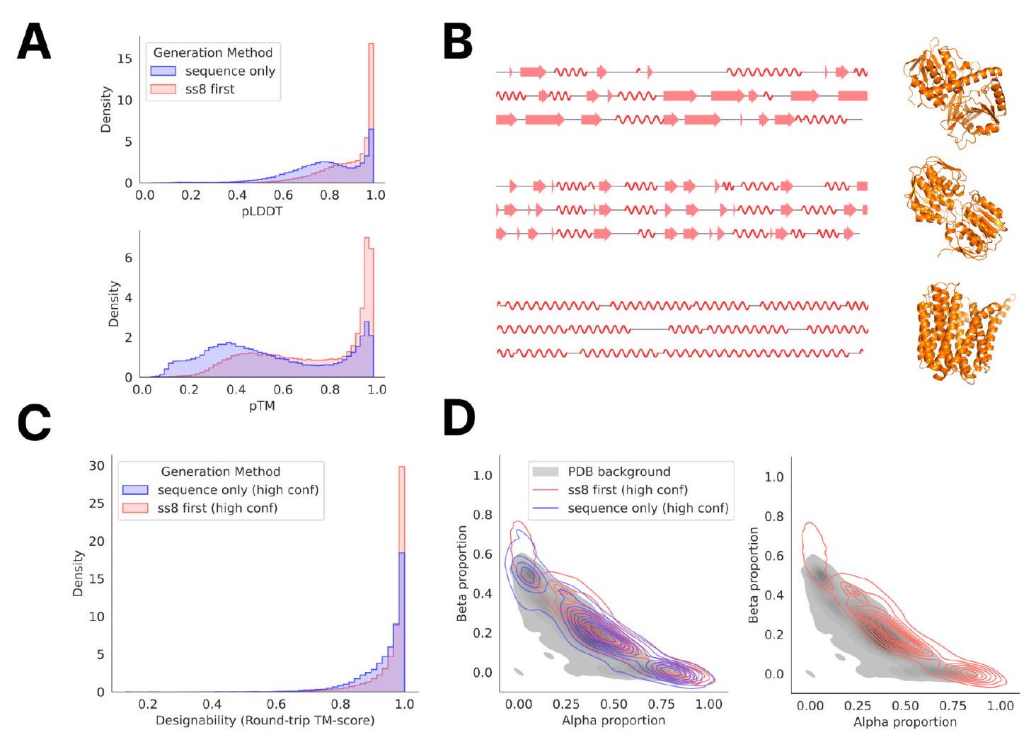
e tokens, then amino acid sequence with the ESM3 7B model. (A) Distribution of mean pLDDT and pTM of sequences generated by chain-of-thought ("ss8 first") compared to directly generating the sequence ("sequence only"). (B) Sample generations of SS8 tokens and the predicted structure of its corresponding CoT sequence. (C) TM-score between predicted structures of high-confidence ( $\mathrm{pTM}>0.8$, mean pLDDT $>0.8$ ) generated sequences and their corresponding inverse folded, then re-folded structures. (D) Comparison of the secondary structure composition of high-confidence generated sequences to the distribution of proteins in the PDB. ment metrics (backbone cRMSD, 3-class secondary structure accuracy, and SASA Spearman $\rho$ ) can be calculated on the relevant span in the ESMFold-predicted structure and the original template protein. Continuing the previous example for the structure track, we would compute the RMSD between residues 20-35 in the ESMFold structure predicted of the ESM3-generated sequence and residues 20-35 of the original test protein. For the function annotation track, we run InterProScan (38) on each generated sequence and extract function keywords from the emitted annotations. We report function keyword recovery at the protein level, computing the proportion of all function keywords in the prompt which appear anywhere in the function keywords from the InterProScan annotations of the generation.
\section*{A.3.8. Steerable Design}
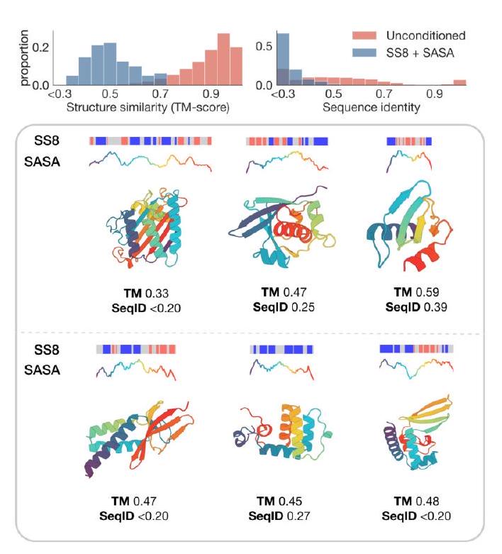
g DSSP, we compute the residue-level SS8 and SASA for each of these proteins to prompt ESM3, masking all other tracks. We show in Fig. S15A that the generated proteins are diverse, globular, and closely follow the SS8 and SASA prompts while having no close sequence or structure neighbors in the training set. Interestingly, these proteins are not folded with high confidence or accuracy by ESMFold (mean pTM 0.44 , mean TM-score to reference 0.33), suggesting that these are challenging proteins to fold. The ESM3generated sequences have a similar confidence (mean pTM 0.45 ) but much higher accuracy (mean TM-score 0.64).
Second, we classify the residue-level secondary structure for a set of eight symmetric protein backbones using DSSP. These proteins were previously designed using ESMFold $(5,91)$ and have varying secondary structure (alpha and beta) and varying symmetries (5-fold and 8 -fold). Again, ESM3 is able to design these proteins successfully with high confidence ( $\mathrm{pTM}>0.8$, pLDDT $>0.8$ ) and low sequence similarity to the training set Fig. S15B. The structural similarity is moderate for these designs due to the high structural conservation of the protomer units in each design. All designs are generated using a constant temperature of 0.7 with $\mathrm{L} / 2$ decoding steps, where $\mathrm{L}$ is the protein length. We sample 256 sequences for each prompt and filter generations by pTM ( $>0.8$ ), pLDDT ( $>0.8$ ), and accuracy in satisfying the SS8 prompts ( $>0.8$ ). Final examples were selected from these filtered designs by visual inspection. Sequence similarity to the training set was computed using the same procedure as the unconditional generations, and structure similarity was computed using Foldseek (39) in TM-score mode (alignment-type 1) with sensitivity -s 7.5.
\section*{A.3.9. Composing Prompts}
with novel characteristics. To demonstrate this, we augment the standard functional motif scaffolding task (i.e., partial structure and sequence prompts) with additional conditioning to specify the type of scaffold for ESM3 to design. The functional sites comprise a combination of ligand binding sites coordinated by residues remote in sequence and those defined by short local motifs. For each motif, the coordinates and amino acid identities of all residues from the reference PDB structures are input to the model, with random shuffling and augmentation of the gaps between each active site. See Appendix A.4.5 for a description of this augmentation procedure and the specifications of the ligand-binding sites chosen. In addition to these sites, we also create a set of 12 partial sequence and structure prompts derived from conserved functional motifs (Table S10). These motifs are defined using a combination of the benchmark dataset in Watson et al. (23) and conserved sequence patterns from the Prosite database (92).
The scaffold conditioning is defined using either SS8 tokens (to specify secondary structure composition) or function keywords defined by InterPro accession numbers (to specify a particular fold). For each combination of functional site and scaffold prompt, we sample between 256 and 2048 times to generate proteins with diverse and novel characteristics. All designs were generated with the 7B-parameter model, a constant temperature of 0.7 , and $L / 2$ decoding steps for a protein of length $L$.
HHHH $\mathrm{HHHHH}$ $\mathrm{HH}$ and a beta-alpha-beta prompt might look like EEEHHHHH_EE, where H is a residue within an alpha helix and $\mathrm{E}$ is a residue in a beta strand. We then combine this with the augmented partial structure and sequence tracks given by a functional site motif. To increase the diversity of the scaffolds and maximize the probability of generating physically realizable prompt combinations, we generate between 256 and 1024 designs for each combination of SS8 and functional site motif. For each generation, we uniformly sample a random length $L$ between 150 and 400 . Then, we produce a set of secondary structure spans with length 5-20 residues, each separated
A
B
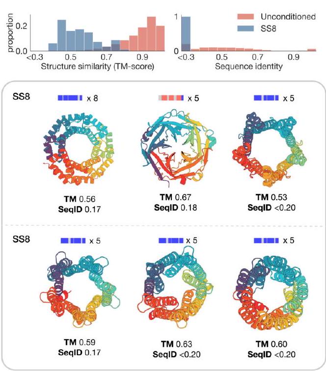
Figure S15. Prompting ESM3 to generalize beyond its training distribution. (A) Proteins designed using SS8 and SASA prompts derived from recent structures in the PDB with low structural similarity to the training set. Prompts along the protein length are visualized above each generation; secondary structure is shown using three-class (alpha $=$ blue, beta $=$ orange, coil $=$ gray) and SASA is shown as a line plot colored by residue index to match the cartoon below. (B) Symmetric proteins designed using SS8 prompting. Histograms show the similarity to the nearest training set protein by structure (TM-score) and sequence (sequence identity) compared to unconditional generation.
\begin{tabular}{rccc} \hline Motif & PDB ID & Chain ID & PDB Residue Identifiers \ \hline ACE2 binding & $6 \mathrm{vw} 1$ & $\mathrm{~A}$ & $19-89,319-366$ \ Ferredoxin & $6 \mathrm{6} 6 \mathrm{r}$ & $\mathrm{A}$ & $1-44$ \ Barstar binding & $7 \mathrm{mrx}$ & $\mathrm{B}$ & $25-47$ \
19-28$ \ PD-1 binding & $5 \mathrm{ius}$ & $\mathrm{A}$ & $63-83,119-141$ \ DNA-binding helix-turn-helix & $11 \mathrm{cc}$ & $\mathrm{A}$ & $1-52$ \ P-loop & $5 \mathrm{ze} 9$ & $\mathrm{~A}$ & $229-243$ \ Double EF-hand & $1 \mathrm{a} 2 \mathrm{x}$ & $\mathrm{A}$ & $103-115,139-152$ \ Lactate dehydrogenase & $11 \mathrm{db}$ & $\mathrm{A}$ & $186-206$ \ Renal dipeptidase & $1 \mathrm{itu}$ & $\mathrm{A}$ & $124-147$ \ Ubiquitin-activating enzyme E1C binding & $1 \mathrm{yov}$ & $\mathrm{B}$ & $213-223$ \ DNA topoisomerase & $1 \mathrm{a} 41$ & $\mathrm{~A}$ & $248-280$ \ \hline \end{tabular}
Table S10. Functional motif definitions for conserved regions. by a gap of 3-10 residues, such that the total length adds up to $L$. Finally, to avoid incompatibility between the partial structure and secondary structure constraints, we also mask the SS8 tokens at positions where structure is specified by the functional site prompt. Secondary structure-prompted designs was assessed by running DSSP on the designed sequence and measuring the fraction of prompted residues which were assigned the correct secondary structure. Success was determined by a pTM $>0.8$, all-atom cRMSD $<$ 1.5 for the functional site, and SS8 accuracy $>0.8$.
overed $>0$.
We assess novelty of each motif-scaffold combinations by measuring the TM-score between the generated scaffold and the chain from which the motif is derived (Table S12). This confirms that the model is not retrieving the original motif scaffold, particularly for secondary structure-prompted scaffolds where we do not provide any explicit instructions to produce diverse designs. For the motifs derived from ligand binding residues (magnesium, serotonin, calcium, zinc, protease inhibitor 017, and Mcl-1 inhibitor YLT), we additionally use Foldseek to search the PDB for any other proteins which share that motif (as defined by BioLiP (93)), as a more stringent evaluation of novelty. For all but zincbinding and magnesium-binding motifs, Foldseek finds no significant hits at an E-value threshold of 1.0. The hits discovered for zinc and magnesium have only modest TMscore ( 0.76 and 0.64 ), demonstrating that the model still finds novel scaffolding solutions for these ligands. To assess whether the generated scaffolds are likely to be designable, we measure a self-consistency TM-score under orthogonal computational models by inverse-folding the designed structure with ESM-IF (94) (using a temperature of 0.5 ) and re-folding with ESMFold (5). We report the best scTM over 8 inverse folding designs in Table S12.
\section*{A.3.10. Multimodal Editing Examples}
he left-to-right ordering of the catalytic triad in the template trypsin. 128 prompts were generated by this procedure. Each of these prompts was combined with a function keyword prompt derived from the template protein, specifically InterPro (38) tags IPR001254 (serine proteases, trypsin domain) and IPR009003 (peptidase S1, PA clan), to arrive at a final set of 128 prompts. The base ESM 7B model was then prompted to generate the sequence of the remaining 147 residues of the protein conditioned on the randomly placed catalytic triad sequence and structure coordinates and function keywords. $L=150$ decoding steps were used with a temperature of 0.7 , with 32 generations per prompt. Generations were then filtered by active site cRMSD, ESM3 pTM, and InterPro Scan keyword outputs, with the generation shown in Fig. 2D selected finally by visual inspection.
Generation quality was measured using ESMFold (5) pTM of the generated sequence, in addition to self-consistency. For self-consistency, we inverse fold the ESM3-predicted structure of the generation with ESM-IF1 (94) 8 times and re-fold with ESMFold, reporting the mean and std of the TM-scores between the 8 ESMFold-predicted structures and the ESM3-predicted structure. To perform a blast search of the sequence, we use a standard Protein Blast search (51). We set the max target sequences parameter to 5000 and sort results by sequence length and sequence identity, selecting the first sequence that is a serine protease. This yields the reference WP_260327207 which is 164 residues long and shares $33 \%$ sequence identity with the generation.
ordinates from this region are placed in the prompt at the same residue indices, to prompt ESM3 to generate the same helix. This is composed with a SASA prompt of 40.0 for each of the 11 helix residues, prompting ESM3 to place this helix on the surface of the protein. Finally, we prompt with the secondary structure of 5 central beta strands surrounding the buried helix, residues 33-36, 62-65, 99-103, 125-130, and 179-182. ESM3 7B is then used to generate 512 protein sequences conditioned on this prompt using $\frac{L}{2}$ decoding steps and a temperature of 0.7. Designs are filtered by ESM3 pTM and adherence
\begin{tabular}{|c|c|c|c|} \hline Scaffold & Reference & InterPro tags & Total Length \ \hline Beta propeller & $8 \sin \mathrm{A}$ & \begin{tabular}{l} IPR001680 (1-350) \ IPR036322 (1-350) \ IPR015943 (1-350) \end{tabular} & 353 \ \hline TIM barrel & $7 \mathrm{rpnA}$ & \begin{tabular}{l} IPR000652 (0-248) \ IPR020861 (164-175) \ IPR035990 (0-249) \ IPR013785 (0-251) \ IPR000652 (2-249) \ IPR022896 (1-249) \end{tabular} & 252 \ \hline MFS transporter & 4ikvA & \begin{tabular}{l} IPR011701 (1-380) \ IPR020846 (1-380) \ IPR036259 (1-380) \end{tabular} & 380 \ \hline Immunoglobulin & $7 \mathrm{sbdH}$ & \begin{tabular}{l} IPR036179 (0-116; 124-199) \ IPR013783 (0-206) \ IPR003597 (124-202) \ IPR007110 (0-115; 121-207) \ IPR003599 (6-115) \ IPR013106 (11-114) \end{tabular} & 209 \ \hline Histidine kinase & 8dvqA & \begin{tabular}{l} IPR003594 (47-156) \ IPR003594 (47-158) \ IPR004358 (118-137) \ IPR004358 (141-155) \ IPR004358 (101-112) \ IPR005467 (0-158) \ IPR036890 (4-159) \ IPR036890 (3-156) \end{tabular} & 166 \ \hline Alpha/beta hydrolase & 7yiiA & \begin{tabular}{l} IPR029058 (0-274) \ IPR000073 (26-265) \end{tabular} & 276 \ \hline \end{tabular}
Table S11. InterPro tags extracted from CAMEO test set proteins for prompting with fold specification.
\begin{tabular}{rrcc} & & & \
riginal) & Designability (scTM) \ \hline 017 & beta & 0.264 & 0.967 \ ACE2 & alpha & 0.606 & 0.871 \ CA & Immunoglobulin & 0.441 & 0.781 \ MG & ab-hydrolase & 0.293 & 0.969 \ TIM-barrel & 0.328 & 0.980 \ Renal-dipeptidase & alpha-beta-alpha & 0.644 & 0.933 \ SRO & mfs-transporter & 0.345 & 0.992 \ Topoisomerase & histidine-kinase & 0.269 & 0.948 \ YLT & alpha-beta & 0.229 & 0.899 \ ZN & alpha & 0.567 & 0.996 \ \hline \end{tabular}
Table S12. Novelty and designability metrics. Metrics are shown for motif scaffolds shown in Fig. 2C. Novelty is measured by computing the TM-score to the original scaffold from which the motif is derived. Designability is measured by self-consistency TM-score over eight samples by inverse folding with ESM-IF and refolding with ESMFold. All designs are distinct from their original scaffolds while retaining high designability. to the SASA prompt. The final generation is chosen by visual inspection. The generation is evaluated as described above (ESMFold pTM 0.71, scTM mean 0.82, std 0.045). Examining the generation, ESM3 is able to satisfy the input constraints: the generated protein maintains the structure of the helix (cRMSD $0.18 \AA$ ) and the alternating alpha-beta fold (both the generation and the template have 7 strands alternating with helices), while exposing the helix motif to the surface (mean SASA $28.35 \AA^{2}$ ). Furthermore, the generation is structurally distinct: a Foldseek search (39) of AlphaFold-DB, ESMAtlas, and PDB in TM-align mode reveals no hit with TM-score greater than .76.
ixed at 7 residues. Each helix and strand region is then separated by 3 mask tokens, with a mask token appended to the $\mathrm{N}$ and $\mathrm{C}$ termini of the prompt as well. This yields a secondary structure prompt of total length 159 , which is combined with a function keyword prompt derived from the reference protein: keywords are derived from IPR013785 (aldolase-type TIM barrel) and IPR000887 (KDPG/KHG aldolase). ESM3 7B is then used to generate 256 samples with $L$ decoding steps and a temperature of 0.7 . The design shown is chosen by filtering by ESM3 pTM and visual inspection. In the second step, the secondary structure prompt from the first step is expanded to contain 11 helix-strand subunits, for a total prompt length of 225 residues (4 mask tokens are now appended to the $\mathrm{N}$ and $\mathrm{C}$ termini, rather than just 1). ESM3 7B is then used to generate 256 samples with $L$ decoding steps and a temperature of 0.7 , with generations filtered by ESM3 pTM and visual inspection. The generation is evaluated as described above (ESMFold pTM 0.69, scTM mean 0.97, std 0.011). The generation is structurally distinct: a Foldseek search (39) of AlphaFold-DB, ESMAtlas, and PDB in TM-align mode reveals no hit with TM-score greater than . 61 .