Since the introduction of RLHF (40) there have been a number of algorithms developed to tune large models trained via unsupervised learning to better follow instructions and generally align their generations to user preferences (41, 42, 95, 96). We use IRPO (Iterative Reasoning Preference Optimization) due to its simplicity in implementation and good performance. The IRPO loss combines supervised finetuning with contrastive learning from preference pairs. IRPO operates on a dataset $\mathcal{D} \sim\left(y{w}, y{l}, x\right)$ consisting of prompt $x$ and a pair of completions $y{w}$ (preferred) and $y{l}$ (not preferred). It also operates on two separate models: the reference model $\pi{\text {ref }}$ and the current model $\pi{\theta}$. The reference model $\pi{\text {ref }}$ is the fixed base model of the same scale, and the current model $\pi{\theta}$ is the model being optimized.
$$ \begin{align} \mathcal{L}{\mathrm{IRPO}}\left(\pi{\theta} ;\right. & \left.\pi{\mathrm{ref}}\right)=\mathcal{L}{\mathrm{NLL}}+\alpha \mathcal{L}{\mathrm{DPO}}= \ & -\mathbb{E}{\left(x, y{w}, y{l}\right) \sim \mathcal{D}}\left[\frac{\log \pi{\theta}\left(y{w} \mid x\right)}{\left|y{w}\right|+|x|}+\right. \ \alpha \log \sigma & \left.\left(\beta \log \frac{\pi{\theta}\left(y{w} \mid x\right)}{\pi{\mathrm{ref}}\left(y{w} \mid x\right)}-\beta \log \frac{\pi{\theta}\left(y{l} \mid x\right)}{\pi{\mathrm{ref}}\left(y_{l} \mid x\right)}\right)\right] \tag{2} \end{align} $$
The IRPO loss contains two terms. The $\mathcal{L}{\text {NLL }}$ term maximizes the $\log$ likelihood of the preferred example normalized by the length of the sequence, providing signal to reinforce the good generations from the model. The $\mathcal{L}{\text {DPO }}$ term is the contrastive preference tuning term, which increases the difference in log likelihoods between the preferred and not preferred examples while staying close to the reference model (41). The use of the reference model serves as a regularizer to prevent overfitting to the preference dataset, which can often be small. There are two hyperparameters, $\alpha$ and $\beta$. $\alpha$ weights the relative importance of the supervised with the preference loss and the $\beta$ parameter controls how close we stay to the reference model: the higher the beta, the closer we stay. We minimize this loss with respect to the current model parameters $\theta$.
ESM3 is a multi-modal model so the prompt can be any combination of the input tracks of (partial) sequence, structure, and function and the generation y can be any of the output tracks. In our experiments we always generate the amino-acid sequence so this will be our running example from now on. Since an amino-acid sequence $y$ can be generated from prompt $x$ in many multi-step ways computing the full likelihood $\pi(y \mid x)$ would involve integrating over all possible multi-step decoding paths. Since this is intractable, we use a surrogate that mirrors pre-training, shown in Eq. (3) and described below.
$$ \begin{equation} \log \pi(y \mid x) \approx \mathbb{E}{m}\left[\sum{i \in m} \log p\left(y{i} \mid y{\backslash m}, x\right)\right] \tag{3} \end{equation} $$
To approximate the likelihood of a generation $y$ from prompt $x$, we mask $y$ with a mask sampled from a linear noise schedule, prompt ESM3 with $\left{y_{\backslash m}, x\right}$, and compute the cross-entropy of ESM3 logits with the masked positions of $y$. During training, the same mask is used to compute the likelihoods for the reference policy vs current policy, as well as for the preferred sample vs non preferred sample.
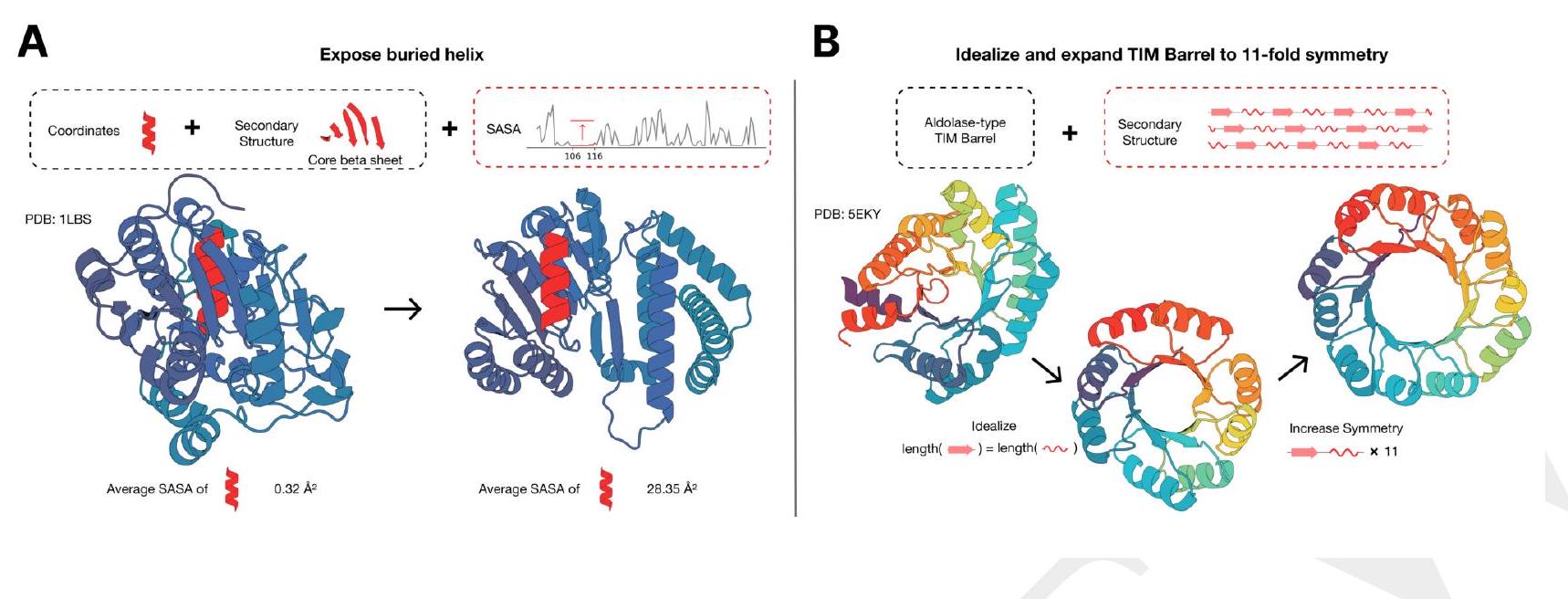
Figure S16. Multimodal protein editing with ESM3. (A) ESM3 exposes a buried helix in an protein while maintaining the alternating alpha-beta sandwich fold of the protein. (B) ESM3 is used in a two-step iterative edit, where first secondary structure prompting and function prompting are used to idealize a reference TIM barrel. Secondary structure prompting is then used to increase the number of subunits in the TIM barrel from 8 to 11 .
Rearranging the DPO term of the loss function gives some insight into how it finetunes the model for the preference pairs. $$ \begin{align} \mathcal{L}{\mathrm{DPO}}\left(\pi{\theta} ;\right. & \left.\pi{\mathrm{ref}}\right)= \ & \mathbb{E}{\left(x, y{w}, y{l}\right) \sim \mathcal{D}}\left[-\log \sigma\left(-\beta z{\theta}\left(x, y{l}, y{w}\right)\right)\right] \tag{4} \end{align} $$ where $$ \begin{aligned} z{\theta}\left(x, y{l}, y{w}\right) & =\log \frac{\pi{\theta}\left(y{l} \mid x\right)}{\pi{\mathrm{ref}}\left(y{l} \mid x\right)}-\log \frac{\pi{\theta}\left(y{w} \mid x\right)}{\pi{\mathrm{ref}}\left(y{w} \mid x\right)} \ & =\log \frac{\pi{\mathrm{ref}}\left(y{w} \mid x\right)}{\pi{\mathrm{ref}}\left(y{l} \mid x\right)}-\log \frac{\pi{\theta}\left(y{w} \mid x\right)}{\pi{\theta}\left(y{l} \mid x\right)} \end{aligned} $$
The function $f(z)=-\log \sigma(-\beta z)=\log (1+\exp (\beta z))$ is the softplus function, and is an approximation of the hinge function; in other words $f(z)=\beta z$ when $z>>0$ and $f(z)=0$ when $z \ll 0$. Because of this property, there are two cases. In the case where $$ \begin{equation} \log \frac{\pi{\mathrm{ref}}\left(y{w} \mid x\right)}{\pi{\mathrm{ref}}\left(y{l} \mid x\right)}>>\log \frac{\pi{\theta}\left(y{w} \mid x\right)}{\pi{\theta}\left(y{l} \mid x\right)} \tag{5} \end{equation} $$ $f(z)$ is in the linear regime, so the loss function is simply maximizing the likelihood ratio $\log \frac{\pi{\theta}\left(y{w} \mid x\right)}{\pi{\theta}\left(y{l} \mid x\right)}$. In the case where $$ \begin{equation} \log \frac{\pi{\text {ref }}\left(y{w} \mid x\right)}{\pi{\text {ref }}\left(y{l} \mid x\right)} \ll \log \frac{\pi{\theta}\left(y{w} \mid x\right)}{\pi{\theta}\left(y{l} \mid x\right)} \tag{6} \end{equation} $$ the loss has saturated. This ensures that we do not deviate too far from the reference model.
These dynamics also hold true in the case of ESM3 finetuning. Although we use a surrogate instead of the true likelihood, the loss will increase the surrogate of the preferred pair over the non preferred pair until the current model deviates too much from the reference model.
Possibly the most important part of preference tuning is to decide how to bucket generations into preferences. The desired objectives for a generation are quality and correctness. Quality refers to the viability of the sequence to be a stable protein. Correctness refers to the extent to which it follows the given prompt; also called prompt consistency. This section only deals with structure coordinate prompts, so prompt consistency can be measured via constrained site RMSD (cRMSD), which is the RMSD between the prompt coordinates and the corresponding coordinates in the predicted structure of the generated sequence. Sequence quality can be measured via predicted-TM (pTM) of a structure predictor on the generated sequence.
As with any metric, especially one which is really a surrogate such as a structure predictor, there is a risk of over optimizing: the model keeps improving the specific metric e.g. in our case pTM but the actual property of interest, the viability of the sequence to be a stable protein, stops correlating with the metric (97). Using orthogonal models to rank our training dataset vs to perform evaluation helps mitigate this.
To create the training datasets, generations are evaluated according to cRMSD and pTM of ESM3 7B to maintain a consistent structure predictor across all datasets. After the preference tuning phase, the generations from the tuned models are evaluated with ESMFold cRMSD and pTM as an orthogonal model. Training on ESM3 derived metrics while evaluating on ESMFold derived metrics should reduce the risk of over optimization for adversarial generations.
All ESM3 model scales are trained with the IRPO loss (Eq. (2)) on their respective preconstructed training datasets consisting of structure coordinate prompts and generations of various difficulty. The datasets have 16 generations each for 30,000 prompts from the respective ESM3 model. Preference selection is determined via a threshold of metrics. A sample is considered "good" if it has ESM3 7B pTM $>0.8$ and backbone cRMSD to its structure prompt $<1.5 \AA$.
Each "good" sample is paired with a "bad" sample to create a preference pair. We found that enforcing a gap between metrics of paired generations improves results, so to qualify as a "bad" sample the generation must have a delta $\mathrm{pTM}=\mathrm{pTM}{\text {good }}-\mathrm{pTM}{\text {bad }}>=0.2$ and delta backbone $c R M S D=c R M S D{\text {good }}-c^{2} M S D{\text {bad }}<-2 \AA$. Each prompt can have multiple preference pairs, and prompts with no valid preference pair are discarded.
The structure prompts are composed of a variety of proteins adapted from our pre-training pipeline. $50 \%$ of the prompts are synthetic active sites, while the other $50 \%$ are structure coordinates randomly masked with a noise schedule. All of the structure prompts are derived from PDB structures with a temporal cutoff of before May 1st, 2020.
The synthetic active sites are derived by finding sequences from PDB with coordinating residues. For these structures, the amino acid identities are included in the prompt.
The remaining structure track prompts are masked according to a cosine noise schedule. $50 \%$ of the noise scheduled prompts are masked in completely random positions, and the other $50 \%$ are masked according to an autocorrelation mechanism that prefers sequentially masked positions.
Each model's training dataset consists of generations of its own reference model. For each prompt, we generate samples from the corresponding ESM3 model scale using iterative decoding with $L / 4$ steps, where $L$ is the length of the prompt. We anneal the temperature from 1.0 to 0.5 over the decoding steps.
Atomic coordination tasks require the generation of proteins which satisfy challenging tertiary interaction constraints. The model is prompted with the sequence and coordinates of a set of residues which are near in 3D space, but distant in sequence. To evaluate performance on these tasks, we curate a dataset of 46 proteins with ligand binding sites from the Biolip dataset (93). All selected proteins were deposited in the PDB after the training set cutoff date (2020-12-01). The coordinating residues shown to the model are given by the ligand binding sites defined in the Biolip dataset (Table S13).
ESM3 is prompted with the sequence and coordinates of the residues for a particular ligand binding site. We ask ESM3 to generate novel structures by applying multiple transformations to the prompt. The total sequence length is sampled evenly to be 150,250 , or 350 residues (regardless of the original sequence length). Next, we define a contiguous span of coordinating residues to be prompt residues with fewer than 5 sequence positions between them. The order and the distance between contiguous spans of residues is shuffled. Together, this ensures that, for example, the original protein will no longer satisfy the prompt. We consider a generation a success if backbone cRMSD $<1.5 \AA$ and $\mathrm{pTM}>0.8$.
We construct a total of 1024 prompts for each ligand and generate a completion for each prompt with the model we are evaluating. We report Pass@ 128, which is an estimate for the fraction of ligands with at least one successful completion after 128 prompts per ligand. We estimate this using an unbiased estimator (Chen et al. (98), Page 3) using the success rate over 1024 prompts. We visualize randomly selected successful generations for both the base model and finetuned model in Fig. S18
To judge the value of preference tuning, we also train a supervised finetuning (SFT) baseline where we finetune the model to increase likelihood of the high quality samples without the preference tuning loss. The 1.4B, 7B, and 98B models solve $14.2 \%, 33.7 \%$, and $44.6 \%$ of atomic coordination tasks at 128 generations, respectively, which improves upon the base models but is much lower than their corresponding preference tuned versions.
Each IRPO model is trained for 1000 steps using RMSProp. The learning rates are $1 \mathrm{e}-5,1 \mathrm{e}-5$, and $5 \mathrm{e}-6$ for the $1.4 \mathrm{~B}$, $7 \mathrm{~B}$, and 98B, respectively, annealed using a cosine schedule after a 150 step warmup. Gradient norms are clipped to 1.0.
For all IRPO runs $\beta=0.05$ and $\alpha=0.8$. The SFT baseline uses the same hyperparameters, but with $\alpha=0.0$ to disregard the preference tuning term.